Vacation Contamination: Predicting Beach Water Pollution

Beach pollution is a persistent problem leading to serious illness and harming coastal economies. While most cases are not reported, swimming in polluted waters is estimated to cause >3.5 million cases of stomach flu per year in the USA and can be especially dangerous for children, elderly, or individuals with weakened immune systems. Subsequent beach closers impact coastal tourism costing as high as $37k in losses per day. With climate change, increased antibiotic resistance, and population growth, the threat of beach water contamination only gets worse.

In Hawaii, where beaches are integral to local communities and the main driver of the tourism industry, beach water contamination is especially worrisome. To combat this problem, the Hawaii State Department of Health (Clean Water Branch) performs empirical testing for hazardous bacteria at hundreds of sites around the coastline of the Hawaiian Islands. This process is expensive and time consuming, requiring a team of people to visit sites individually to bring samples back to the lab for over-night growth and quantification. Due to limited resources, some sites are sampled once per week, while others are sampled only a few times a year or not at all. Beaches are closed when bacterial levels are discovered to exceed the safety threshold, but due to the low sampling frequency, contamination could persist for many days before the public is warned.

Automated prediction of beach contamination could not only lessen and streamline the workload of the Department of Health but also provide early warning to beach-goes and tourism companies. But what can be used to predict this? While beach water can be contaminated through multiple routes, it commonly occurs from island runoff, leading to increases in beach water turbidity and salinity. Because island runoff occurs during heavy rains, climate and temporal data may be strongly predictive. Measurements of beach water turbidity, salinity, and precipitation are easy to monitor and can be passively collected, which make them ideal data to build my model.

The Data: Bacteria + Climate

To build a model of bacterial contamination in beach water, I first needed to determine when and where contamination has happened in the past. I scraped the Hawaii Department of Health website for data including bacteria levels, water turbiditiy, and salinity measures from 2004-2017 on Oahu, Hawaii’s most populous island. To get a feel of the data, I first created a tableau visualization of bacterial contamination around Oahu. Each dot represents a site that was sampled for that given week, with green representing low and red representing high levels of bacteria. Toggle through the weeks using the slider bar to visualize bacterial levels.

From this visualization, a few things become apparent about this data.

1. Contamination is rare.
2. Locations are very sparsely and unevenly sampled.
3. Contamination is geographically constrained and does not appear to spread.

Furthermore, by visualizing levels of bacteria over time at each site individually, I noticed blooms of bacterial growth over several orders of magnitude. Below, you can see a plot of bacterial levels over time for individual locations. Use the slider bar or the drop-down menu to see how bacterial levels and sampling frequency changes with location.

According to the Department of Health, beach water is unsafe when bacterial levels exceed 130 colonies/100mL of water. Since my goal was to provide predictions about beach water safety, I categorized each sample into two classes depending on whether bacterial levels exceeded the safety threshold.

1. Class 0: Safe (levels <130c/100mL)
2. Class 1: Hazardous (levels >130c/100mL) This allowed me to simplify the problem by reframing it as a classification problem.

Feature Engineering

After converting the bacterial levels in two categories, I could begin to collect and engineer features to predict beach water contamination. By scraping the Hawaii Department of Health website, I obtained measurements of water turbidity and salinity. I used the Dark Sky API to obtain specific climate information for each location and sampling date/time. Because it may take multiple days for island runoff to make it into the beach water, I also obtained climate data for the three days preceding each sampling. Lastly, I converted the time of year into a continuous function, using a sin/cos transformation, to include temporal information into my model. Some of the climate data is slightly correlated, such as precipitation levels and humidity, however many models including decision trees learn very well despite correlated data.

One feature that I specifically choose not to include was location. The Department of Health currently triages its sampling load based off of location alone. In order to insure that my solution was providing additional value, I omitted this information from my model.

Modeling with Imbalanced Data

The next challenge I needed to address before training my model was the imbalance between my two classes in the data. Thankfully, only 2% of the samples collected by the Department of Health contained hazardous levels of bacteria. This makes model training more difficult because simply guessing that the water is never contaminated gives you a very high accuracy. As expected, when I trained models on raw imbalanced training sets, the algorithm learned to predict the majority class (safe) almost every time and almost never identified hazardous samples.

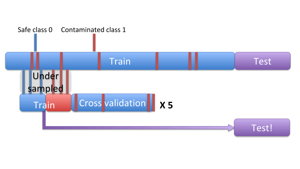
To compensate for class imbalance, I undersampled from my training set to balance the amount of class 0 (safe) and class 1 (unsafe) in my final training data. While this solution greatly decreases the false negative rate (chance of missing a hazardous sample), it also increases the false positive rate (predicting a hazardous sample when it is actually safe). For this particular application, a low false negative rate is required for this algorithm to be useful and while not ideal, a few false positives are acceptable as they can still be weeded out by empirical testing.

The following image shows a schematic of Undersampling, inspired from https://mangarella.github.io/BreatheFree/:

Picking an Algorithm

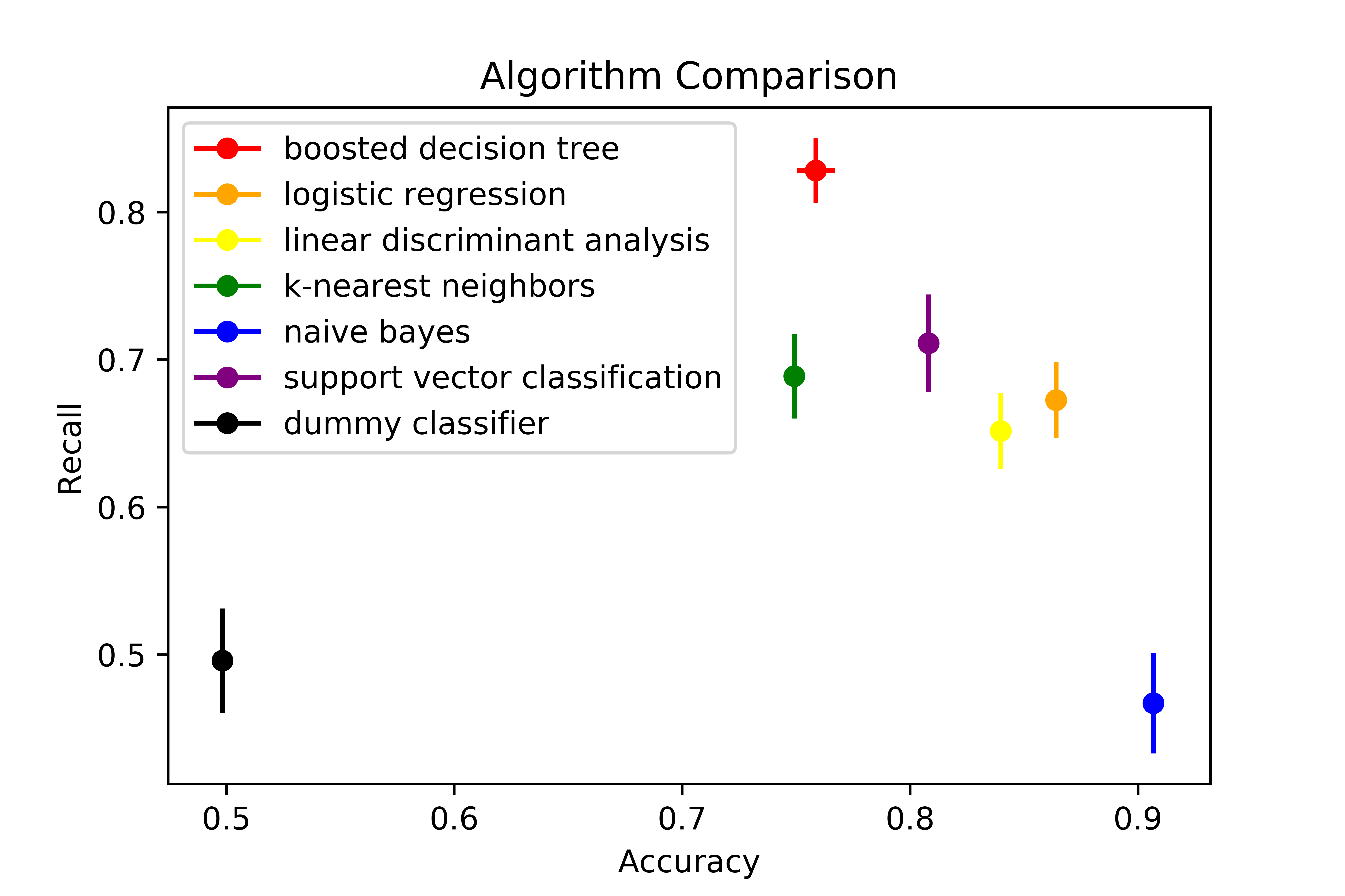
Now that I have classified by data into two classes, collected and engineered my features, and generated a balanced training set, my data is ready for machine learning. But what algorithm should I use? Using python’s sklearn, I can easily try many algorithms. For this particular case, I compared each algorithm using the metrics I cared about, recall (true positive rate) and accuracy. While many algorithms resulted in similar results, reporting around 70%-80% recall and similarly high accuracy, I ended up choosing Gradient Boosted Decision Trees because they are non-parametric, robust in the face of correlated data, and most importantly, had a high true positive rate and easy routes to identify feature importance.

The following figure compares the algorithms:

Evaluating the Model

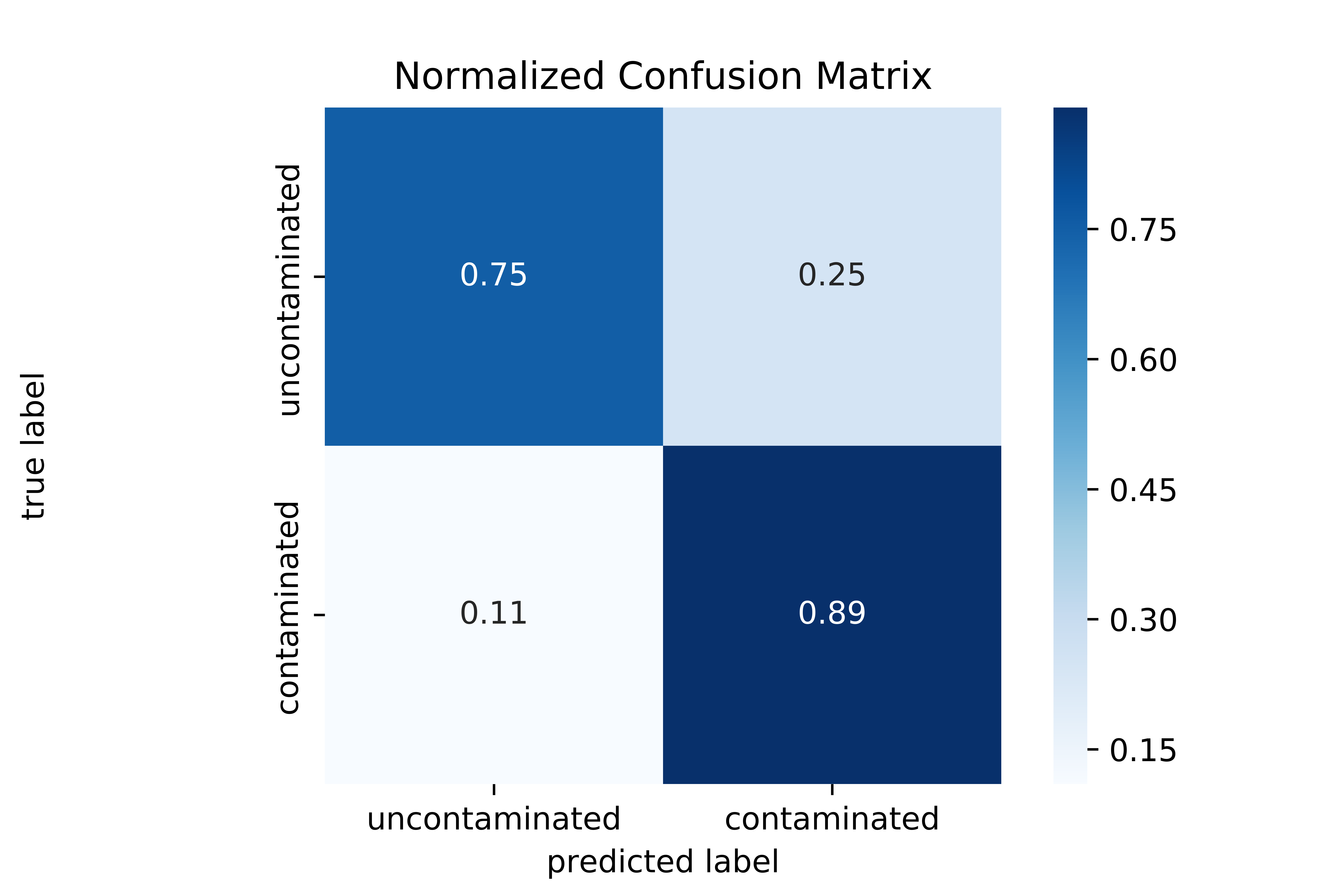
Looking more closely with a confusion matrix, I can really start to evaluate the model. The Gradient Boosted Tree gave great results as the model correctly predicts the majority of all the hazardous samples (with 89% recall). While the false positive rate is higher than would be desirable, the model still successfully identifies 75% of all safe samples correctly. Taken together, following this model would reduce the sampling workload of the Department of Health by over 1/3rd.

Here is the confusion matrix:

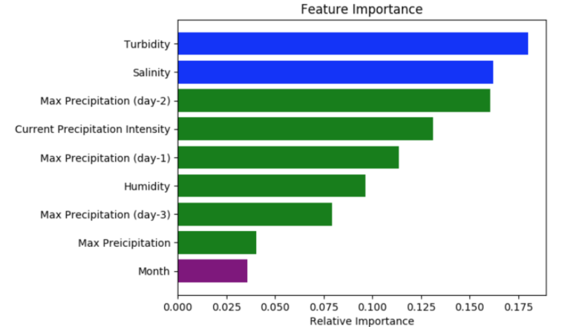
Not surprisingly, the top features are the direct measures of the water, the water turbidity and salinity. The next most important feature is the max precipitation at two days prior to the sampling. This also makes sense, given that it may take multiple days for rainwater to carry island runoff into the beach water. Interestingly the time of year feature (“Month”) had very low importance, which may be because Hawaii does not have traditional seasons.

The following shows feature importance:

Summary and Future Directions

In summary, I’ve created a model that accurately predicts bacterial contamination in Hawaii’s beach water with a true positive rate of 89%. Sampling according to this model would reduce the workload by over 1/3rd. The development of this project spanned only 3 weeks at Insight as a results there are many interesting avenues that I did not have time to explore.

Additional Features

Since these hazardous bacteria are naturally found in human and animal excrement, the beach’s proximity to cesspools and sewer lines could play an important role in its probability of contamination. Popular beaches with heavy human usage could also lead to higher levels of contamination. Additionally, beach water movement could dilute out the hazardous bacteria, suggesting that current strength and waves could be an important features.

Model at Large

While this data was trained and tested specifically on Hawaii beach water data, I am interested in how this model could be transferred to other locations. In this case, the feature importance may change. For example, the time of year could become more important, depending on the seasonality of the location, and the time delay between predictive rain and sampling could change, depending on the geography.

Acknowledgements

This project was developed as part of my participation in the Insight Data Science Fellows Program. Many thanks to my fellow Fellows for their insights and help in the development of this project.